


In the following is given some examples from the 8 different topics mentioned. Unfortunately, most of the work has been confidential, but the chosen examples should give an idea of the interdisciplinary nature of biosimulation.
1. Biosimulation
* Quantitative biology, virtual experiments, virtual patients, disease life cycle
BIOLOGICAL EXPERIMENT
VIRTUAL EXPERIMENT
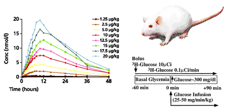
- A biological experiment starts with an animal/patient and an experimental protocol. The results show, for example, the plasma concentration as a function of time for different doses of a drug.
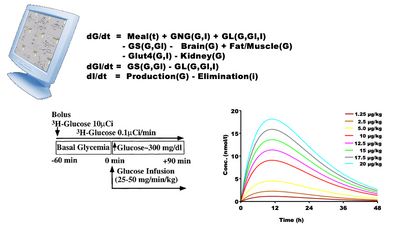
- A virtual experiment is a series of equations that hopefully describe the biology investigated. The protocol is the same, so the model gives a proposed set of plasma curves.
- A coincidence between the two set of curves may indicate, but not prove, that the mechanisms in the model are understood correctly.
- So model analysis must be regarded as a supplement to experiments or trials - and vice versa.
2. Exploratory data analysis
* Mechanisms behind patterns in data, Complex non-normal statistics, Aplied mathematics,
Generating hypotheses, Graphical presentation
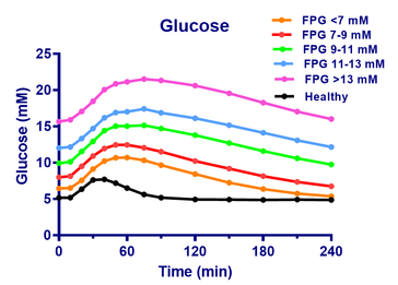
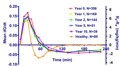
- The figure show the glucose and insulin concentrations from meal tolerance tests (MTT’s) of healthy and of Type 2 patients at first visit.
- The patients are divided into 5 groups after fasting glucose values (FPG), and the curves show the mean glucose values of each group.
- The curves are almost parallel in spite of the large differences in fasting glucose, so there appears to be a ”universal” shape of the meal response for Type 2 patients.
- The glucose change rate, dG/dt, is estimated as (Gn-Gn-1)/(tn-tn-1). Assuming a glucose distribution volume of 16 L and a body weight of 70 kg, the estimated dG/dt in mM/min is converted to the difference between glucose appearence rate, Ra, and disappearance rate, Rd (Ra-Rd) in mg/kg/min (right y-axis).
- The curves are almost identical from year to year. It appears that the fluxes are independent of treatment type, dose etc.
- On the other hand, the relation for the healthy is markedly different. There is a transient upstroke-downstroke, followed by is a steady state, where influx and outflux of glucose are equal.
- So a simple, exploratory data analysis reveals new insight in Type 2 diabetes.
3. Pharmacokinetics and -dynamics
* Mechanisms behind ADME of medicines, Receptor kinetics, Transport phenomena, Albumin binding etc. Interaction between kinetics and dynamics
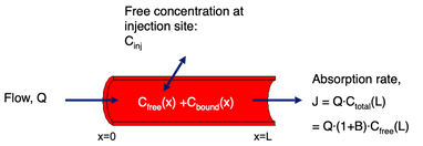
Albumin bound insulin: Insulin diffuses over the capillary wall and is carried away by the blood stream.
The capillary concentration, C(x)=Cfree(x)+Cbound(x), increases as the blood passes the injection site.
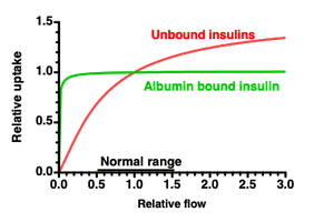
A small flow gives almost equilibrium at the veneous end, so flow determines the uptake.
A large flow keeps the concentration low, so diffusion over the capillary wall is limiting.
For albumin bound insulins more than 98% can bind to albumin, so albumin acts as a buffer that keeps the free plasma concentration Cfree(x) low, so the difference Cinj-Cfree(x) is kept large.
The result is a lower variation and a lower risk of hypoglycemic events.
4. Antibodies:
* Immune responses, epitope optimization, Fab’s and other fragments, sweeping antibodies, biacore analysis, interplay between surface bound and free
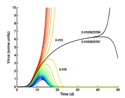
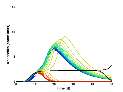
Covid 19: A model is constructed, where exponential virus multiplication is counteracted by an exponentially increasing, but delayed, immune response.
Due to the delay, the initial virus exposure (seed) is crucial. Small seeds (blue to green) are defeated rapidly and may be symptomless. Larger seeds (yellow to dark red) give increasing severity. Over a certain threshold, the infection may be lethal.
The figure shows how the disease is prolonged as the seed approaches the borderline between 0.018 and 0,019 units.
The black curve shows the borderline. After more than a month, a difference of 1 in 184 mill. determins the end result.
The subtle balance between virus and antibody elimination is shown in the lower figure. A as the seed approaches the critical limit, the response is more and more delayed.
At small seeds (blue to green), the antibodies win and forces an elimination of the virus, wherafter the amount of antibodies slowly declines.
At large seeds (yellow to dark red), the virus wins and forces a total elimination of the antibodies, whereafter the virus increases to high and dangerous levels.
At the borderline (black), they are on equal footing, and a small disturbance can determine the outcome.
5. Pathophysiology
* Physiological mechanisms behind diseases, disease progression, treatment strategies
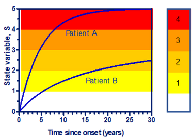
- The development of late diabetic complications can be described via a state variable, S, that increases over time, until it saturates after some decades.
- As the state variable increases, the complications increase, and via the doctor’s diagnoses, levels with increasing severity are passed.
- Some patients only progress to a low steady level, while other reach very high levels with severe complications.
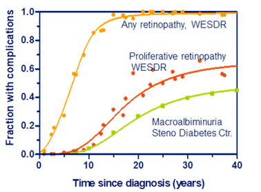
- The model is compared with the WESDR (Wisconsin Epidemiologic Study of Diabetic Retinopathy)-study and results from Steno Diabetes Center.
- The three patient groups, A: Type 1, B:Type 2 using insulin, and C: Type 2 not using insulin, are assumed to have a normally distributed steady level with a certain mean, Smax, and SD.
- The model gives the following results: A: Smax=3.5±10%, B: Smax=2.8±21%, and C: Smax=2.8±29%. Similarly, the level for any retinopathy is: 2.2±12%, proliferative retinopathy: 3.24±12%, Macroalbuminamia: 3.53±13%.
- This is very low SD’s for clinical trials, so the development of late diabetic complications seem to follow simple and predictable rules.
6. Control theory
* Hormonal and neural control, metabolism control, predictability, nonlinear dynamics,
and complexity theory.
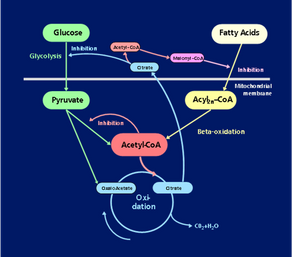
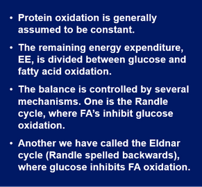
- The balance between glucose and fatty acid oxidation is controlled by the mitochondria.
- The control involves two mechanisms. One is the Randle cycle, where fatty acids inhibit glucose oxidation.
- Another - equally important – we have called the Eldnar cycle (Randle spelled backwards), where glucose inhibits the oxidation of fatty acids.
- In the fasting state, most glucose goes to the brain, so the other organs mainly burn fatty acids, and the Randle cycle prevents the cells from using glucose.
- With high glucose, as after a meal, the breakdown of fat is inhibited, and many cells burn glucose.
- With overfeeding, the Eldnar cycle switch to building fatty acids from glucose. The fatty acids are then transported to the fat cells and stored.
7. Biomedical physics
* Nuclear medicine, radiation physics, cell- and molecular biology, medical devices, drug administration

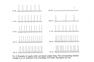
- To study the information processing in nerve cells, two glass microelectrodes were inserted into a nerve cell. The electrodes were provided with “negative capacity” and the possibility of current injection, voltage clamp etc.
- Regular current pulses were injected in one electrode, and the response of the nerve cell was recorded from the other.
- The nerve cell does not respond on every pulse but responds with a pulse pattern that either is regular (left) or chaotic (right).
- As the current strength is increased, the cell reacts on more and more pulses, so the mean frequency increases, but the patterns shift between regular and irregular in a complex way.
- The signal transmission between nerve cells is thus not just relaying pulses, or a sum of pulses, from one cell to another like the setup in a so-called neural network.
- Instead, the nerve cell is itself an advanced computer.
8. Regulatory affairs
• Mechanisms behind effects and side effects, benefit-risk of medicines, patient adherence
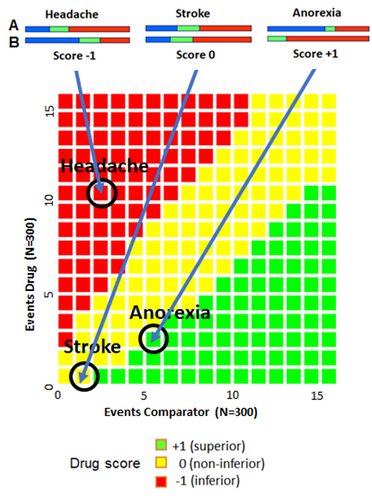
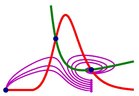
- To compare the benefits and risks of two drugs, A and B, a special diagram, based on confidence intervals, can be used.
- This is particularly useful, when the data are sparse.
- First, the confidence interval score for different benefits or risks, here side effects, are determined as shown in the upper figures.
- Taking drug B as the comparator, the score depends on the confidence intervals (green). If all points of the interval for B is above those for A, the score is -1, meaning that A is inferior to B.
- If all points of the interval for B is below all those for A, the score is +1, meaning that A is superior to B.
- If the two intervals overlap – even for a short distance – the score is 0, meaning that A is non-inferior to B.
- In the present case, A is superior regarding anorexia, non-inferior regarding stroke, but inferior regarding headache.
- By weighting the different effects/side effects, a combined score can be achieved. This is used to compare different trials.
+45 5178 8999
mcj@biosimconsult.dk
Morten Colding-Jørgensen
CVR No. 33687311